Facts About Excel If Formula Uncovered

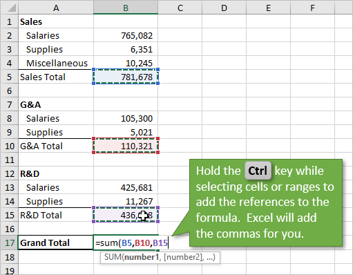
By pushing ctrl+shift+facility, this will compute and return worth from multiple varieties, rather than simply specific cells included in or increased by one an additional. Computing the sum, product, or quotient of private cells is easy-- simply use the =SUM formula as well as go into the cells, worths, or variety of cells you want to execute that arithmetic on.

If you're looking to find total sales earnings from numerous offered devices, as an example, the range formula in Excel is ideal for you. Here's exactly how you 'd do it: To start making use of the range formula, kind "=AMOUNT," and in parentheses, go into the initial of two (or 3, or 4) varieties of cells you want to increase with each other.

This stands for multiplication. Following this asterisk, enter your 2nd series of cells. You'll be multiplying this second variety of cells by the first. Your progress in this formula should now appear like this: =AMOUNT(C 2: C 5 * D 2:D 5) Ready to push Go into? Not so quick ... Because this formula is so difficult, Excel reserves a different keyboard command for varieties.

This will certainly identify your formula as a range, covering your formula in support personalities and effectively returning your item of both arrays integrated. In income calculations, this can reduce your effort and time significantly. See the final formula in the screenshot over. The MATTER formula in Excel is represented =MATTER(Begin Cell: End Cell).

As an example, if there are eight cells with gotten in worths in between A 1 as well as A 10, =COUNT(A 1: A 10) will certainly return a worth of 8. The MATTER formula in Excel is specifically valuable for big spread sheets, where you wish to see the amount of cells consist of actual entrances. Do not be deceived: This formula will not do any kind of mathematics on the worths of the cells themselves.

What Does Excel Formulas Mean?

Utilizing the formula in bold above, you can quickly run a count of active cells in your spread sheet. The outcome will look a something such as this: To do the ordinary formula in Excel, get in the worths, cells, or series of cells of which you're calculating the average in the layout, =AVERAGE(number 1, number 2, and so on) or =AVERAGE(Start Value: End Worth).

Finding the standard of a series of cells in Excel keeps you from having to locate private sums and after that performing a different department equation on your total. Making use of =STANDARD as your first message entrance, you can let Excel do all the help you. For referral, the average of a team of numbers is equal to the amount of those numbers, separated by the number of products because team.

This will certainly return the sum of the worths within a wanted array of cells that all satisfy one standard. For example, =SUMIF(C 3: C 12,"> 70,000") would certainly return the sum of values in between cells C 3 and C 12 from only the cells that are better than 70,000. Allow's claim you desire to establish the profit you produced from a checklist of leads who are related to particular area codes, or calculate the amount of certain staff members' salaries-- but just if they drop over a certain quantity.

With the SUMIF function, it does not need to be-- you can quickly accumulate the sum of cells that meet certain standards, like in the income example over. The formula: =SUMIF(array, criteria, [sum_range] Range: The array that is being evaluated utilizing your criteria. Criteria: The criteria that establish which cells in Criteria_range 1 will certainly be included with each other [Sum_range]: An optional variety of cells you're mosting likely to build up along with the very first Array entered.

In the instance listed below, we wanted to compute the amount of the incomes that were more than $70,000. The SUMIF feature built up the buck quantities that surpassed that number in the cells C 3 through C 12, with the formula =SUMIF(C 3: C 12,"> 70,000"). The TRIM formula in Excel is signified =TRIM(text).

The Main Principles Of Sumif Excel

For instance, if A 2 consists of the name" Steve Peterson" with unwanted spaces before the very first name, =TRIM(A 2) would return "Steve Peterson" without any rooms in a new cell. Email and file sharing are remarkable tools in today's work environment. That is, up until among your associates sends you a worksheet with some actually funky spacing.

Rather than painstakingly removing and including areas as required, you can clean up any uneven spacing utilizing the TRIM feature, which is made use of to remove additional areas from information (other than for single rooms between words). The formula: =TRIM(message). Text: The message or cell from which you wish to eliminate spaces.

To do so, we got in =TRIM("A 2") right into the Solution Bar, as well as reproduced this for every name listed below it in a brand-new column next to the column with undesirable rooms. Below are some other Excel solutions you could find useful as your information management needs expand. Allow's claim you have a line of text within a cell that you intend to break down right into a few various segments.

Objective: Utilized to draw out the first X numbers or personalities in a cell. The formula: =LEFT(text, number_of_characters) Text: The string that you desire to remove from. Number_of_characters: The variety of personalities that you wish to extract starting from the left-most character. In the example below, we went into =LEFT(A 2,4) right into cell B 2, and duplicated it right into B 3: B 6.

Function: Utilized to draw out personalities or numbers between based on placement. The formula: =MID(text, start_position, number_of_characters) Text: The string that you wish to draw out from. Start_position: The placement in the string that you wish to start drawing out from. As an example, the very first setting in the string is 1.

What Does Learn Excel Mean?

In this example, we went into =MID(A 2,5,2) into cell B 2, and also replicated it right into B 3: B 6. That enabled us to extract both numbers beginning in the fifth placement of the code. Purpose: Made use of to remove the last X numbers or characters in a cell. The formula: =RIGHT(message, number_of_characters) Text: The string that you wish to remove from.

excel formulas between sheets excel formula x to the power of y excel formulas not showing